Kunstig intelligens (IT-2702) - høst 2006. Forelesning 7 Emner: Usikkerhetsbehandling - Utvidelse av standard logikk - Den klassiske ”certainty factor”

Presentasjon om: "Kunstig intelligens (IT-2702) - høst 2006. Forelesning 7 Emner: Usikkerhetsbehandling - Utvidelse av standard logikk - Den klassiske ”certainty factor”"— Utskrift av presentasjonen:

1 Kunstig intelligens (IT-2702) - høst 2006. Forelesning 7 Emner: Usikkerhetsbehandling - Utvidelse av standard logikk - Den klassiske ”certainty factor” metoden - Fuzzy mengder - Statistikk-baserte metoder - og spesielt Bayesianske nett - Kunnskapsbaserte metoder

2 Den reelle verden er usikker It is the mark of an instructed mind to rest satisfied with that degree of precision which the nature of the subject admits, and not to seek exactness where only an approximation of the truth is possible.(Aristotle) All traditional logic habitually assumes that precise symbols are being employed. It is therefore not applicable to this terrestrial life but only to an imagined celestial existence.(Bertrand Russell) So far as the laws of mathematics refer ro reality they are not certain. And so far as they are certain they do not refer to reality.(Albert Einstein)

3 Inferens-metoder Deduksjon - sannhetsbevarende slutning - basis er slutningsregelen modus ponens (P(x) -> Q(x)) & P(a) -> Q(a) Klassisk eksempel: (Isa-man(x) -> Is-mortal(x)) &Isa-man(Socrates) ->Is-mortal(Socrates) Abduksjon - ikke sannhetsbevarende - "inference to the best explanation" (P(x) -> Q(x)) & Q(a) ~> P(a) Eksempel: (Has-appendicitis(x) -> Has-abdominal-pain(x)) &Has-abdominal-pain(Socrates) ~>Has-appendicitis(Socrates)

4 Ikke-monotone systemer Forutsetninger for 1. ordens predikatlogikk: - komplett domenebeskrivelse - konsistent domenebeskrivelse - monotont voksende kunnskapsbase I ikke-monotone systemer er en eller flere av disse forutsetningene ikke oppfylt. Logikk-tilnærminger: Modal-operatorerunless, is-consistent-with, … Truth Maintenance systemerJTMS, ATMS,... AndreCWA, Circumscription,...

5 Modal-operatorer : p(X) unless q(X) => r(X) good-student(X) ^ M study-hard(X) => graduates(X) is-consistent-with Set cover approach: En abduktiv forklaring på et sett av fakta (S2) er et annet sett av fakta (S1) som er tilstrekkelig for å forårsake S2. En optimal forklaring er det minimale sett S1. Logikkbasert approach : En abduktiv forklaring på et sett av observasjoner (O) er det minimale sett av hypoteser (H) som er konsistent med den aktuelle bakgrunnskunnskap (K). O kan ikke være utledbar fra K alene.

6 Usikkerhetsbehandling - Certainy Factors - usikkerhetsanslag i regel-baserte systemer - benyttet i MYCIN og avledede ES-skall - basert på anslag av - degree of beliefMB(H/E) - degree of disbeliefMD(H/E) - som kobineres i en Certainty Factor CF(H/E) = MB(H/E) - MD(H/E)

7 Usikkerhetsbehandling - CF (forts.) - eksempel, Mycin-type regel: IF (P1 and P2) or P3 THENR1 (0.7) and R2 (0.3) - kombinasjon av to regler som peker på samme konklusjon: CF(R1)+CF(R2) - (CF(R1)xCF(R2)) | CF(R1), CF(R2) pos. CF(R1)+CF(R2) + (CF(R1)xCF(R2)) | CF(R1), CF(R2) neg. CF(R1)+CF(R2) 1 - min((abs(CF(R1), abs(CF(R2)) | ellers

8 Usikkerhetsbehandling - Fuzzy Sets - et fuzzy set (fose mendge?) er en mendge der elementene i større eller mindre grad kan sies å være medlem av mendgen - en medlemsskapsfunksjon definerer i hvilken grad (mellom 0 og 1) et element er medlem av mengden - øvelse: tegn medlemsskapsfunksjonene [0,1] for ung og gammel i mendgen av aldre [1,100]. 0 1 205010030701090806040 0.5 1

9 Luger: Artificial Intelligence, 5 th edition. © Pearson Education Limited, 2005 Fig 9.6the fuzzy set representation for “small integers.” 7

10 Luger: Artificial Intelligence, 5 th edition. © Pearson Education Limited, 2005 Fig 9.7A fuzzy set representation for the sets short, medium, and tall males. 8

11 Luger: Artificial Intelligence, 5 th edition. © Pearson Education Limited, 2005 Fig 9.8The inverted pendulum and the angle θ and dθ/dt input values. 9

12 Luger: Artificial Intelligence, 5 th edition. © Pearson Education Limited, 2005 Fig 9.9The fuzzy regions for the input values θ (a) and dθ/dt (b). 10

13 Luger: Artificial Intelligence, 5 th edition. © Pearson Education Limited, 2005 Fig 9.10The fuzzy regions of the output value u, indicating the movement of the pendulum base. 11

14 Luger: Artificial Intelligence, 5 th edition. © Pearson Education Limited, 2005 Fig 9.11The fuzzificzation of the input measures X 1 = 1, X 2 = -4 12

15 Luger: Artificial Intelligence, 5 th edition. © Pearson Education Limited, 2005 Fig 9.10The Fuzzy Associative Matrix (FAM) for the pendulum problem. The input values are on the left and top. 13

16 Luger: Artificial Intelligence, 5 th edition. © Pearson Education Limited, 2005 14

17 Luger: Artificial Intelligence, 5 th edition. © Pearson Education Limited, 2005 Fig 9.13The fuzzy consequents (a) and their union (b). The centroid of the union (-2) is the crisp output. 15

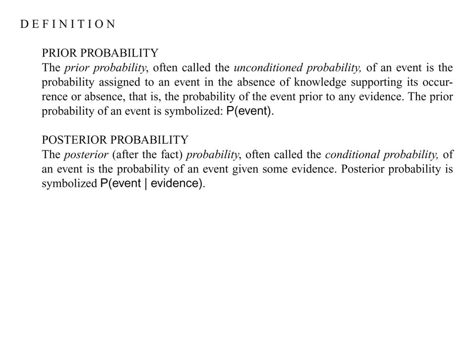
18 Usikkerhetsbehandling - Statistiske metoder Basisbegreper: Prior probability (a priori sanns., ubetinget sanns.) Sannsynligheten, P, for en hendelse, A, uten at noe informasjon er gitt:P(A) Posterior probability (a posteriori sanns., betinget sanns.) Sannsynligheten, P, for en hendelse, A, gitt informsjonen E:P(A/E) Kombinasjon av uavhengige (ubetingede) sanns. P(A & B) = P(A) x P(B)

19

20 Probability theory, the general form of Bayes’ theorem

21 The application of Bayes’ rule to the car purchase problem: Luger: Artificial Intelligence, 5 th edition. © Pearson Education Limited, 2005 23

22 Naïve Bayes, or the Bayes classifier, that uses the partition assumption, even when it is not justified: Luger: Artificial Intelligence, 5 th edition. © Pearson Education Limited, 2005 24

23 Luger: Artificial Intelligence, 5 th edition. © Pearson Education Limited, 2005 Fig 5.4The Bayesian representation of the traffic problem with potential explanations. Table 5.4 The joint probability distribution for the traffic and construction variables of Fig 5.3. 25

24 Fig 9.14The graphical model for the traffic problem, first introduced in Section 5.3. Luger: Artificial Intelligence, 5 th edition. © Pearson Education Limited, 2005 19

25 Luger: Artificial Intelligence, 5 th edition. © Pearson Education Limited, 2005 20

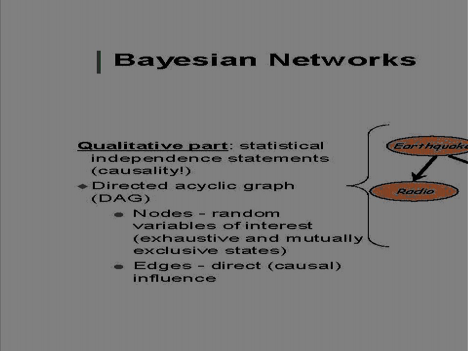
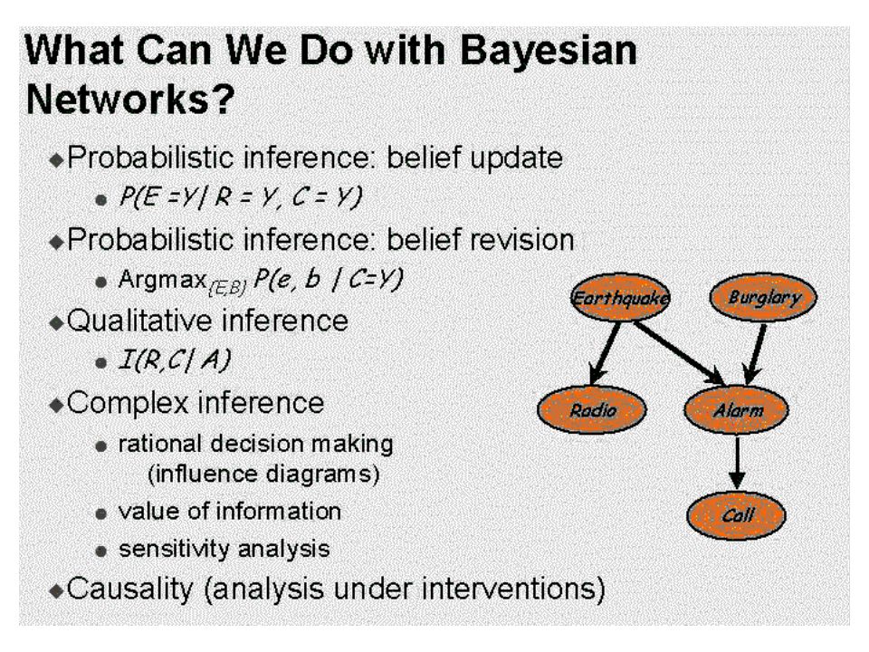
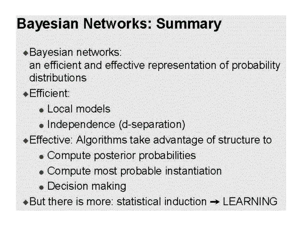
26 = Belief Networks

27

28 Defining the d-separation of nodes in a belief network (after Pearl 1988) Another way to express the same thing: Nodes are independent of their non-descendants given their parents.

29 B A C E R C B A E A If Known OR (d-separated) (d-connected)

30 Fig 9.15a is a serial connection of nodes where influence runs between A and B unless V is instantiated. 9.15b is a diverging connection, where influence runs between V’s children, unless V is instantiated. In 9.15c, a converging connection, if nothing is known about V the its parents are independent, otherwise correlations exist between its parents. Luger: Artificial Intelligence, 5 th edition. © Pearson Education Limited, 2005 21

31 Rød kule: Verdien er kjent (gjelder for de tre siste eksempeluttrykkene)

32 Fig 9.16An example of a Bayesian probabilistic network, where the probability dependencies are located next to each node. This example is from Pearl (1988). Luger: Artificial Intelligence, 5 th edition. © Pearson Education Limited, 2005 24

33 Luger: Artificial Intelligence, 5 th edition. © Pearson Education Limited, 2005 Table 9.4 The probability distribution for p(WS), a function of p(W) and p(R) given the effect of S. We calculate the effect for x, where R = t and W = t. 23

34 Luger: Artificial Intelligence, 5 th edition. © Pearson Education Limited, 2005 A junction tree algorithm. 25

35 Fig 9.17A junction tree (a) for the Bayesian probabilistic network of (b). Note that we started to construct the transition table for the rectangle R, W. Luger: Artificial Intelligence, 5 th edition. © Pearson Education Limited, 2005 26

36

37

38

39 Fig 9.18A Markov state machine or Markov chain with four states, s 1,..., s 4 Luger: Artificial Intelligence, 5 th edition. © Pearson Education Limited, 2005 27

40 Luger: Artificial Intelligence, 5 th edition. © Pearson Education Limited, 2005 28

41 Luger: Artificial Intelligence, 5 th edition. © Pearson Education Limited, 2005 29

42 Luger: Artificial Intelligence, 5 th edition. © Pearson Education Limited, 2005 30

43 Fig 9.19A hidden Markov model of two states designed for the coin flipping problem. The a ij values are determined by the elements of the 2 x 2 transition matrix. Luger: Artificial Intelligence, 5 th edition. © Pearson Education Limited, 2005 31

44 Fig 9.20A hidden Markov model for the coin flipping problem. Each coin will have its own individual bias. Luger: Artificial Intelligence, 5 th edition. © Pearson Education Limited, 2005 32

45 Fig 9.21A PFSM representing a set of phonemically related English words. The probability of each word occurring is below that word. Adapted from Jurasky and Martin (2000). Luger: Artificial Intelligence, 5 th edition. © Pearson Education Limited, 2005 33

46 Luger: Artificial Intelligence, 5 th edition. © Pearson Education Limited, 2005 34

47 Fig 9.22A trace of the Viterbi algorithm on the paths of Fig 9.21. Rows report the maximum value for Viterbi on each word for each input value (top row). Adapted from Jurafsky and Martin (2000). Luger: Artificial Intelligence, 5 th edition. © Pearson Education Limited, 2005 35

48 Usikkerhetsbehandling - Forklaringsbasert - modell-basert tilnærming - kausale relasjoner oftest benyttet, men også andre relasjoner - relasjonene i modellen antas usikre, og kan ha ”degree of belief” anslag - usikkerhet begrenses ved multiple forklaringer, dvs. en hypotese støttes i større eller mindre grad av forklaringene som genereres i modellen eks. ABEL (Stanford), HeartFailureModel (MIT), ”Endorsement Theory” (UMass), CREEK (NTNU-IDI)